Multi-Scale Statistics
An ecological network may look modular or nested depending on the scale at which it is observed (see Flores et al 2013 for an example). For example, if we focus at the global scale of the network we may infer that the network is modular and not nested. However, if we go to the inner community modules (after performing one of the modularity algorithms) we may discover that they are actually nested. Performing this kind of analysis may be exhausting, specially if nothing is to be found. However, BiMat provides the tools for performing a first exploratory analysis that we call Multi-scale Statistics.
Under this kind of analysis, BiMat first find what are the modular structure of the network. Once we found what are the modules, BiMat treat them as independent networks by performing a meta-statistics analsyis on them. Finally, if the user have available data about node classification, this data can be used by BiMat to analyze if the modular structure may be explained by node classification (i.e. nodes from the same class may be clustered inside the same module). In order to do that BiMat can make use of two kind of diversity indexes that can be applied to row and/or column modules:
- Simpson's Index of Diversity : $1 - \frac{\sum_{i=1}^c n_i (n_i -1)}{N (N-1)}$
- Shannon's Index of Diversity: $-\sum_{i=1}^c \frac{n_i}{N} \log \frac{n_i}{N}$
where (assuming it will be used on the row species) $c$ is the number of modules, $n_i$ the number of row species belonging to module $i$, and $N$ the number of row species.
Contents
Example: Moebus Meta-scale analysis
In this example we will describe how to perform this kind of statistical analysis in a network that is large enough. This network is composed of 286 bacteria vs 215 phages that represents the largest cross-infection study to date. The phages and bacteria strains were collected across multiple geographical locations across the Atlantic ocean (and we will use this locations as node classes). We will see that this network is modular at the global scale (entire network) but the modules are inded nested. For more information about the analysis of this dataset, the user may want to read our original paper: Flores et al 2013.
Creating the Bipartite object
We need to start by creating our Bipartite object
load moebus_data.mat;
The loaded data contains the bipartite adjacency matrix of the Moebus and Nattkemper study, where 1's and 2's in the matrix represent either clear or turbid lysis spots. It also contains the labels for both bacteria and phages and their geographical location (classes) from which they were isolated across the Atlantic Ocean.
bp = Bipartite(moebus.weight_matrix);    % Create the main object
bp.row_labels = moebus.bacteria_labels;  % Updating node labels
bp.col_labels = moebus.phage_labels;
bp.row_class = moebus.bacteria_stations;   % Updating node ids
bp.col_class = moebus.phage_stations;
We can print the general properties of the network with:
bp.printer.PrintGeneralProperties();
General Properties
	 Number of species:       	   501
	 Number of row species:   	   286
	 Number of column species:	   215
	 Number of Interactions:  	  1332
	 Size:                    	 61490
	 Connectance or fill:     	 0.022
Performing some modularity and nestedness analysis
We can now perform the standard modularity and nestedness calculation. For modularity:
bp.community = LeadingEigenvector(bp.matrix);
% The next flag is exclusive of Newman Algorithm and what it does is to
% performn a final tuning after each sub-division (see Newman 2006).
bp.community.DoKernighanLinTunning = true; % Default value
We need to calculate the modularity explicitly by calling:
bp.community.Detect();
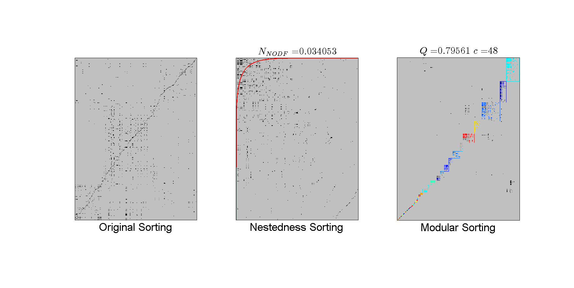
Modularity:
	Used algorithm:             	  LeadingEigenvector
	N (Number of modules):      	                  48
	Qb (Standard metric):       	              0.7956
	Qr (Ratio of int/ext inter):	              0.8348
For nestedness
%Just apply the default (which is NODF)
bp.nestedness.Detect();
Nestedness NODF:
	NODF (Nestedness value):    	              0.0341
	NODF (Rows value):          	              0.0368
	NODF (Columns value):       	              0.0293
Plotting the matrix
Plotting in Matrix Layout You can print the layout of the original, nestedness and modular sorting. If you matrix is weighted in a categorical way using integers (0,1,2...) you can visualize a different color for each interaction (as in this case), but we will turn off this default value:
figure(1);
%Matlab command to change the figure window;
set(gcf,'Position',[0, 72, 1835, 922]);
bp.plotter.use_type_interaction = false; % TURN OFF color matrix cells by weights
bp.plotter.use_labels = false; % plot the node labels
bp.plotter.back_color = [192, 192, 192]/255; % low gray
%After changing all the format we finally can call the plotting functions.

%Original sorting
subplot(1,3,1);
bp.plotter.PlotMatrix();
xlabel('Original Sorting','fontsize',26);

% Nestedness sorting;
subplot(1,3,2);
bp.plotter.use_isocline = true; %The NTC isocline will be plotted.
bp.plotter.isocline_color = 'red'; %Decide the color of the isocline.
bp.plotter.PlotNestedMatrix();
title(['$N_{NODF} = $',num2str(bp.nestedness.N)],...
    'interpreter','latex','fontsize',23)
xlabel('Nestedness Sorting','fontsize',26);

% Modularity
subplot(1,3,3);
bp.plotter.PlotModularMatrix();
title(['$Q = $',num2str(bp.community.Qb),' $c = $', num2str(bp.community.N)],...
    'interpreter','latex','fontsize',23);
xlabel('Modular Sorting','fontsize',26);
Multi-scale part
It is evident that the entire network is modular (a result confirmed by the use of the modularity significance detection suite). Of relevance here is that internal nodes seems to have nested structure, e.g., there is triangular pattern with most of the links above the isocline. Hence, the Moebus network may have multi-scale structure properties (indeed, this was already demonstrated in Flores et al 2013)). Using BiMAT, we can evaluate the internal structure of modules. For example, to evaluate nestedness, BiMat makes use of the InternalStatistics class by treating each of the modules independent networks:
%Focus on the first 15 modules
bp.internal_statistics.idx_to_focus_on = 1:15;
%Perform a default internal analysis
bp.internal_statistics.TestInternalModules();
bp.internal_statistics.meta_statistics...
             .plotter.PlotNestednessValues();
bp.internal_statistics.meta_statistics...
             .plotter.PlotNestedMatrices();
Testing Matrix: 1 . . .
Testing Matrix: 2 . . .
Testing Matrix: 3 . . .
Testing Matrix: 4 . . .
Testing Matrix: 5 . . .
Testing Matrix: 6 . . .
Testing Matrix: 7 . . .
Testing Matrix: 8 . . .
Testing Matrix: 9 . . .
Testing Matrix: 10 . . .
Testing Matrix: 11 . . .
Testing Matrix: 12 . . .
Testing Matrix: 13 . . .
Testing Matrix: 14 . . .
Testing Matrix: 15 . . .
The meta_statistics property is an instance of the class MetaStatistics, which translates to be able to use any of the methods inside MetaStatistics (including its property plotter) in the internal modules. This feature is a reflection of the use of OOP in developing BiMat.
Finally, another multi-scale analysis that BiMat can perform is to quantify if a relationship exists between node labels and module distribution. This feature is of particular use when the node information is available, e.g., with respect to their study origin or other categorical (i.e,. non-metric) feature. If there is a perfect correlation between label and module, then every node inside the same module will share the same label. If there is no relationship, then node labels in a module should be randomly distributed. BiMat makes use of both Shannon's and Simpson's indexes to analyze the label variation inside and between modules. Hence, the heterogeneity of label indices is measured within each module. Then, node labels are randomly swapped, generating an ensemble from which to compare the measured correlation. The next lines will show how to perform this with analysis for the column (phage) nodes: Given the labeling this method calculates the diversity index of the labeling inside each module and compare it with random permutations of the labeling across the matrix.
%Using the labeling of bp and 1000 random permutations
bp.internal_statistics.TestDiversityColumns( ...
    1000,moebus.phage_stations,@Diversity.SHANNON_INDEX);
%Print the information of column diversity
bp.printer.PrintColumnModuleDiversity();
Diversity index:    	  Diversity.SHANNON_INDEX
Random permutations:	                     1000
Module,index value,  zscore,percent
     1,     2.4873, -1.9234,    2.8
     2,     1.9722, -1.5282,    3.6
     3,     2.2497, -5.9533,      0
     4,     1.4791, -5.7535,      0
     5,     1.8174, -6.1189,      0
     6,     1.6094, 0.59588,   28.7
     7,     1.0906, -8.9942,      0
     8,     1.0042, -5.5915,      0
     9,     1.4942, -2.9425,    0.2
    10,     1.7479,-0.51217,   10.7
    11,    0.45056, -8.4525,      0
    12,     1.7678, -3.0172,    0.2
    13,     1.3322, -1.3108,      3
    14,      1.677, -2.4457,    0.7
    15,     1.0397, -2.0111,    0.8
    16,     1.0986, 0.30702,    8.8
    17,          0,     NaN,      0
    18,          0,     NaN,      0
    19,          0,     NaN,      0
    20,    0.63651, -3.0214,    0.1
    21,          0,     NaN,      0
    22,          0,     NaN,      0
    23,          0, -5.4972,      0
    24,    0.69315, 0.19035,    3.5
    25,          0,     NaN,      0
    26,          0,  -5.029,      0
    27,          0,     NaN,      0
    28,          0,     NaN,      0
    29,          0,     NaN,      0
    30,          0,     NaN,      0
    31,          0,     NaN,      0
    32,          0,     NaN,      0
    33,          0,     NaN,      0
    34,          0,     NaN,      0
    35,          0,     NaN,      0
    36,          0,     NaN,      0
    37,          0,     NaN,      0
    38,          0,     NaN,      0
    39,          0,     NaN,      0
    40,          0,     NaN,      0
    41,          0,     NaN,      0
    42,          0,     NaN,      0
    43,          0,     NaN,      0
    44,          0,     NaN,      0
    45,          0,     NaN,      0
    46,          0,     NaN,      0
    47,          0,     NaN,      0
    48,          0, -5.3276,      0