Nestedness
Contents
Description
Nestedness describes the extent to which interactions form ordered subsets of each other. There are several indices for quantifying nestedness bimat implements two of the most commonly used methods, namely, NTC (Nestedness Temperature Calculator) (see Atmar et al 1993) and NODF (for Nestedness metric based on Overlap and Decreasing Fill) (see Almeida-Neto et al 2008)
NODF
The NODF measure normalizes for matrix size, and thus allows matrices of different sizes to be compared. The nestedness range is $0 \le NODF \le 1$, where 0 indicates a matrix of blocks (i.e perfect modular, identity, checkerboard) and 1 corresponds to a perfectly nested structure. NODF is based on two properties: decreasing fill and paired overlap. NODF measures nestedness across rows by assigning a value $M_{ij}^{\text{row}}$ to each pair $i$, $j$ of rows in the interaction matrix: \begin{equation} M_{ij}^{\text{row}} = \begin{cases} 0 & \text{if $k_i \le k_j$}\\ n_{ij}/\min(k_i,k_j) & \text{otherwise,} \end{cases} \label{eq.Mrows} \end{equation} where $k_i$ is the number of ones in row $i$, $k_j$ is the number of ones in row $j$, and $n_{ij}$ is the number of shared interactions between rows $i$ and $j$ (so-called paired overlap). Notice that positive contributions to the NODF require pairs of columns satisfying the decreasing fill property, that is, when $k_i > k_j$. A similar term $M_{ij}^{\text{col}}$ is used to compute column contributions. The total nestedness is the sum of columns and row contributions: \begin{equation} N_{NODF} = \frac{\sum_{ij} M_{ij}^{\text{row}} + \sum_{ij} M_{ij}^{\text{col}}} { m(m-1) /2 + n(n-1)/2}. \end{equation}
Matlab vectorization capabilities allows for very efficient calculation of (\ref{eq.Mrows}) (and its column version): \begin{equation} M_{ij}^{\text{row}} = \frac{(\mathbf{r}_i \cdot \mathbf{r}_j) \left(1-\delta(k_i,k_j)\right)} {\min(k_i,k_j)}, \end{equation} where $\mathbf{r_i}$ is a vector that represents the row $i$ of the adjacency matrix, and $\delta(k_i,k_j)=1$ if and only if $k_i=k_j$. By using this notation, (\ref{eq.nodf}) can be expressed in terms of matrix multiplications that exploit the implicit parallelism provided by Matlab (see code for details). Tests indicate that a vectorised formulation of $N_{NODF}$ outperforms sequential approaches (e.g., using loops) by a factor of over 50 times.
Temperature Calculator (NTC)
A `temperature', $T$, of the interaction matrix is estimated by resorting rows and columns such that the largest quantity of interactions falls above the isocline (a curve that will divide the interaction from the non-interaction zone of a perfectly nested matrix of the same size and connectance). In doing so, the value of $T$ quantifies the extent to which interactions only take place in the upper left ($T\approx0$), or are equally distributed between the upper left and the lower right ($T\approx100$). Perfectly nested interaction matrices can be resorted to lie exclusively in the upper left portion and hence have a temperature of 0. The value of temperature depends on the size, connectance and structure of the network. Because the temperature value quantifies departures from perfect nestedness, we define the nestedness, $N_{NTC}$, of a matrix to range from 0 to 1, $N_{NTC}=(100-T)/100$, such that $N_{NTC}=1$ when $T=0$ (in the case of perfect nestedness) and $N_{NTC}=0$ when $T=100$ (in the case when interactions form a ``checkerboard'' when visualized in matrix format).
Example 1: Calculating Nestedness
The next example shows how to detect nestedness using the default algorithm:
matrix = MatrixFunctions.NESTED_MATRIX(20);
bp = Bipartite(matrix);
bp.nestedness.Detect();
Nestedness NODF:
	NODF (Nestedness value):    	              1.0000
	NODF (Rows value):          	              1.0000
	NODF (Columns value):       	              1.0000
We can also change the default algorithm before calculating nestedness, choosing among one of the two options described before:
bp.nestedness = NestednessNTC(matrix);
bp.nestedness.Detect();
Nestedness NTC:
	NTC (Nestedness value):     	              1.0000
	T (Temperature value):      	              0.0000
Further, there is no need to work directly with a Bipartite instance. The user can also chose to work with a Nestedness instance instead:
%By creating an instance and then calculating nestedness
nes = NestednessNODF(matrix);
nes.Detect();
%Or by calling a static method:
nes2 = Nestedness.NODF(matrix);
Nestedness NODF:
	NODF (Nestedness value):    	              1.0000
	NODF (Rows value):          	              1.0000
	NODF (Columns value):       	              1.0000
Nestedness NODF:
	NODF (Nestedness value):    	              1.0000
	NODF (Rows value):          	              1.0000
	NODF (Columns value):       	              1.0000
Example 2: Accesing detailed results
Altough by calculating the nestedness we can already see what are the nestedness results, sometimes we may need to know detailed values. By just typing the name of the Nestedness instance we have access to these values
(
nes2
nes2 =

  NestednessNODF with properties:

           N_rows: 1
           N_cols: 1
                N: 1
           matrix: [20x20 logical]
           n_rows: 0
           n_cols: 0
             done: 1
    print_results: 0
The description of these properties is showed in the next table:
| Property | Algorithm | Description |
|---|---|---|
| N | Both | nestedness value between 0 and 1 |
| matrix | Both | bipartite adjacency matrix |
| n_rows | Both | number of rows |
| n_cols | Both | number of columns |
| done | Both | if nestedness has been already detected |
| print_results | Both | if results will be printed after detection (default true) |
| N_rows | NestednessNODF | nestedness value for rows between 0 and 1 |
| N_cols | NestednessNODF | nestedness value for columns between 0 and 1 |
| T | NestednessNTC | Temperature value between 0 and 1 |
| do_geometry | NestednessNTC | perform geometry calculation? (default true) |
| index_rows | NestednessNTC | row indexes after sorting |
| index_cols | NestednessNTC | colum indexes after sorting |
| connectance | NestednessNTC | connectance (fill) value between 0 and 1 |
| trials | NestednessNTC | number of random initializations (default 5) |
| do_sorting | NestednessNTC | sort matrix before calculating temperature? (default true) |
Now, we can access a property by just typing it:
nes2.N
ans =

     1
Example 3: Different degrees of nestedness
In this example we will calculate the nestedness of three different degrees of nestedness (
%Creating the matrices
matrix_nested = MatrixFunctions.NESTED_MATRIX(20); %perfect nested
matrix_modular = MatrixFunctions.CHECKERBOARD(20,20); %imperfect nested
matrix_middle = MatrixFunctions.MIX_MATRICES(matrix_nested,matrix_modular); %a combination

ntc_nested = Nestedness.NTC(matrix_nested);
ntc_modular = Nestedness.NTC(matrix_modular);
ntc_middle = Nestedness.NTC(matrix_middle);

nodf_nested = Nestedness.NODF(matrix_nested);
nodf_modular = Nestedness.NODF(matrix_modular);
nodf_middle = Nestedness.NODF(matrix_middle);

%Some plot format for all plots
plot_format = PlotFormat();
plot_format.use_labels = false;
plot_format.cell_color = [0,0,176]/255;
plot_format.use_empty_cell = true;
plot_format.cell_empty_color = [200,200,200]/255;
font_size = 16;

%Plotting
figure(1);
set(gcf,'position', [22,52,1181,664]);

subplot(2,3,1);
ylabel('Original Sort', 'FontSize', font_size+4);
title('Low nestedness degree', 'FontSize', font_size);
PlotWebs.PLOT_MATRIX(matrix_modular, plot_format);
subplot(2,3,2);
title('Some nestedness degree', 'FontSize', font_size);
PlotWebs.PLOT_MATRIX(matrix_middle, plot_format);
subplot(2,3,3);
title('High nestedness degree', 'FontSize', font_size);
PlotWebs.PLOT_MATRIX(matrix_nested, plot_format);

subplot(2,3,4);
ylabel('Nestedness Sort', 'FontSize', font_size+4);
PlotWebs.PLOT_NESTED_MATRIX(matrix_modular, plot_format);
xlabel(['$N_{NTC} = ', num2str(ntc_modular.N),'$, $N_{NODF} = ',num2str(nodf_modular.N),'$'],...
    'FontSize',14, 'interpreter','latex');
subplot(2,3,5);
PlotWebs.PLOT_NESTED_MATRIX(matrix_middle, plot_format);
xlabel(['$N_{NTC} = ', num2str(ntc_middle.N),'$, $N_{NODF} = ',num2str(nodf_middle.N),'$'],...
    'FontSize',14, 'interpreter','latex');
subplot(2,3,6);
PlotWebs.PLOT_NESTED_MATRIX(matrix_nested, plot_format);
xlabel(['$N_{NTC} = ', num2str(ntc_nested.N),'$, $N_{NODF} = ',num2str(nodf_nested.N),'$'],...
    'FontSize',14, 'interpreter','latex');
Nestedness NTC:
	NTC (Nestedness value):     	              1.0000
	T (Temperature value):      	              0.0000
Nestedness NTC:
	NTC (Nestedness value):     	              0.0317
	T (Temperature value):      	             96.8287
Nestedness NTC:
	NTC (Nestedness value):     	              0.5383
	T (Temperature value):      	             46.1694
Nestedness NODF:
	NODF (Nestedness value):    	              1.0000
	NODF (Rows value):          	              1.0000
	NODF (Columns value):       	              1.0000
Nestedness NODF:
	NODF (Nestedness value):    	              0.0000
	NODF (Rows value):          	              0.0000
	NODF (Columns value):       	              0.0000
Nestedness NODF:
	NODF (Nestedness value):    	              0.5738
	NODF (Rows value):          	              0.5760
	NODF (Columns value):       	              0.5715
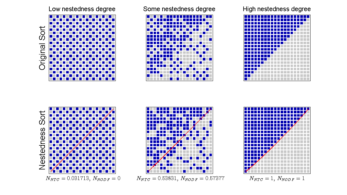
We can see in the plot three different degrees of nestedness using the original sorting (the input without any sorting), and nestedness sorting (in this sorting rows and columns are sorted in decreasing order of their sum totals). First thing to notice is that nestedness sorting only has an effect in matrices that are neither perfectly nested nor imperfectly nested. Further, while NestednessNTC gives a perfect 1 for the perfect nested matrix, it does not give a value of 0 for the imperfect one. The reason behind this number is the way in which NestednessNTC is calculated (which is very sensitive to the final cell positions).