Modularity
Contents
Description
Modularity indicates the presence of dense clusters of related nodes embedded within the network. In many systems, we can find a partition of nodes into specific communities or modules. This modularity metric can be expressed for a bipartite network as: \begin{equation} Q_b = \frac{1}{E} \sum_{ij} \left( B_{ij} - \frac{k_i d_j}{E} \right) \delta(g_i,h_j), \end{equation} where $B_ij$ is the element in the bipartite matrix representing a link (1) or no link (0) between nodes $i$ and $j$, $g_i$ and $h_i$ are the module indexes of nodes $i$ (that belongs to set $R$) and $j$ (that belongs to set $C$), $k_i$ is the degree of node $i$, $d_j$ is the degree of node $j$ and $E$ is the number of links in the network. BiMat contains three algorithms to maximize the last equation, all of them containing different heuristics.
- AdaptiveBrim (Michael J. Barber 2007) : The algorithm uses the BRIM algorithm with an heuristic for looking the optimal value of modules. This heuristic consists in multiply the number of modules $N$ by a factor of two at each interaction as long as the modularity value $Q_b$ continues to increase, at which time the heuristic perform a bisection method between the last values N$ that were visited.
- LPBrim (Xin Liu and Tsuyoshi Murata 2009): The algorithm is a combination between the BRIM and LP algorithms. The heuristic of this algorithms consist in searching for the best module configuration by first using the LP algorithm. The BRIM algorithm is used at the end to refine the results.
- LeadingEigenvector (Mark Newman 2006) : Altough this algorithm was defined for unipartite networks, for certain bipartite networks, this algorithm can give the best optimization. equation, when defined in the unipartite version for two modules, can be expressed as a linear combination of the normalized eigenvectors of the modularity matrix. Therefore, this method divides the network in two modules by choosing the eigenvector with the largest eigenvalue, such that negative and positive components of this eigenvector specifies the division. To implement this algorithm, BiMat first converts the bipartite matrix into its unipartite version.
In addition to optimize the standard modularity $Q_b$ BiMat also evaluates (after optimizing $Q_b$) an a posteriori measure of modularity $Q_r$ introduced in Poisot 2013 and defined as: \begin{equation} Q_r = 2\times\frac{W}{E}-1 \end{equation} where $W = \sum_{ij} B_{ij} \delta(g_i,h_j)$ is the number of edges that are inside modules. Alternatively, $Q_r \equiv \frac{W-T}{W+T}$ where $T$ is the number of edges that are between modules. In other words, this quantity maps the relative difference of edges that are within modules to those between modules on a scale from 1 (all edges are within modules) to $-1$ (all edges are between modules). This measure allows to compare the output of different algorithms.
Example 1: Calculating Modularity
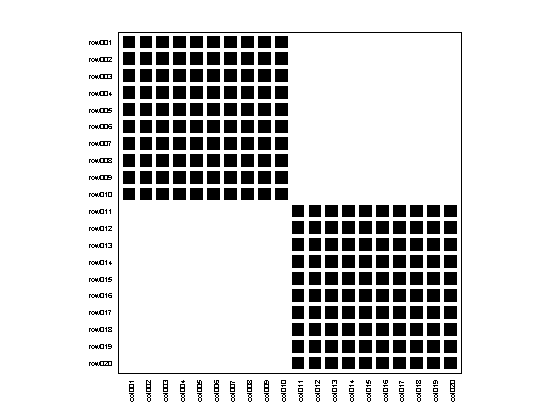
The next example shows how to detect modularity using the default algorithm:
matrix = MatrixFunctions.BLOCK_MATRIX(2,10);
bp = Bipartite(matrix);
bp.plotter.PlotMatrix();
bp.community.Detect();
Modularity:
	Used algorithm:             	        AdaptiveBrim
	N (Number of modules):      	                   2
	Qb (Standard metric):       	              0.5000
	Qr (Ratio of int/ext inter):	              1.0000
We can also change the default algorithm before detecting the community structure, choosing among one of the three options described before:
bp.community = LPBrim(matrix);
bp.community.Detect();
Modularity:
	Used algorithm:             	              LPBrim
	N (Number of modules):      	                   2
	Qb (Standard metric):       	              0.5000
	Qr (Ratio of int/ext inter):	              1.0000
Further, there is no need to work directly with a bipartite instance. The user can also chose to work with a BipartiteModularity instance instead:
%By creating an instance and then calculating modularity
com = LeadingEigenvector(matrix);
com.Detect();
%Or by calling a static method:
com2 = BipartiteModularity.LEADING_EIGENVECTOR(matrix);
Modularity:
	Used algorithm:             	  LeadingEigenvector
	N (Number of modules):      	                   2
	Qb (Standard metric):       	              0.5000
	Qr (Ratio of int/ext inter):	              1.0000
Modularity:
	Used algorithm:             	  LeadingEigenvector
	N (Number of modules):      	                   2
	Qb (Standard metric):       	              0.5000
	Qr (Ratio of int/ext inter):	              1.0000
Example 2: Accesing detailed results
Altough by calculating the modularity we can already see what are the modularity results, sometimes we may need to know detailed values. By just typing the name of the BipartiteModularity instance we have access to these values
(
%A list of all properties
com2
com2 =

  LeadingEigenvector with properties:

    DoKernighanLinTunning: 1
                       Qb: 0.5000
                       Qr: 1
                        N: 2
                   matrix: [20x20 logical]
              row_modules: [20x1 double]
              col_modules: [20x1 double]
                       bb: [20x20 double]
                   n_rows: 20
                   n_cols: 20
                  n_edges: 200
               index_rows: [20x1 double]
               index_cols: [20x1 double]
                   trials: 20
                     done: 1
    optimize_by_component: 0
            print_results: 0
The description of these properties is showed in the next table:
| Property | Algorithm | Description |
|---|---|---|
| Qb | All | standard modularity value between 0 and 1 |
| Qr | All | a-posteriori modularity value between 0 and 1 |
| N | All | number of modules |
| matrix | All | bipartite adjacency matrix |
| row_modules | All | module index for each row |
| col_modules | All | module index for each column |
| bb | All | modularity matrix |
| n_rows | All | number of rows |
| n_cols | All | number of columns |
| n_edges | All | number of edges |
| index_rows | All | row indexes after sorting by modules |
| index_cols | All | column indexes after sorting by modules |
| done | All | if modularity has been already detected |
| optimize_by_component | All | should modularity be optimized by isolated component first? (default false) |
| print_results | All | if results will be printed after detection (default true) |
| trials | AdaptiveBrim/LPBrim | number of initialization trials (default see Options.TRIALS_MODULARITY) |
| prob_reassigment | AdaptiveBrim | probability of reassigment when new modules are created (default 0.5) |
| expansion_factor | AdaptiveBrim | factor of expansion for creating new modules (default 2.0) |
| red_labels | LPBrim | Similar than row_modules |
| col_labels | LPBrim | Similar than col_modules |
| DoKernighanLinTunning | LeadingEigenvector | execute Kernighan tunning after modularity detection? (default true) |
Now, we can access a property by just typing it:
%Number of modules
com2.N
ans =

     2
%Module indices for row nodes
com2.row_modules'
ans =

  Columns 1 through 13

     1     1     1     1     1     1     1     1     1     1     2     2     2

  Columns 14 through 20

     2     2     2     2     2     2     2
%Moudlarity value
com2.Qb
ans =

    0.5000
Example 3: Optimizing at the component level
The default behavior of BiMat is to optimize modularity using the entire adjacency matrix. However, some times the network may have isolated components (sub-graphs with no connections between them). For those instances, the user may want to optimize each sub-graph independent of the others, and then calculate the modularity:
%Loading the data
load data/moebus_data.mat;
%default optimization
bp = Bipartite(moebus.weight_matrix > 0);
bp2.community.optimize_by_component = false;
%sub-graph optimization
bp2 = Bipartite(moebus.weight_matrix > 0);
bp2.community.optimize_by_component = true;
%visualizing the results:
plotFormat = PlotFormat();
plotFormat.back_color = [41,38,78]/255;
plotFormat.cell_color = 'white';
plotFormat.use_labels = false;
subplot(1,2,1);
bp.plotter.SetPlotFormat(plotFormat);
bp.plotter.PlotModularMatrix();
title(['$Q = ', num2str(bp.community.Qb),'$, $N = ',num2str(bp.community.N),'$'],...
    'FontSize',16, 'interpreter','latex');
xlabel('Default Optimization','FontSize', 20);
subplot(1,2,2);
bp2.plotter.SetPlotFormat(plotFormat);
bp2.plotter.PlotModularMatrix();
title(['$Q = ', num2str(bp2.community.Qb),'$, $N = ',num2str(bp2.community.N),'$'],...
    'FontSize',16, 'interpreter','latex');
xlabel('Optimizaing by isolated components','FontSize', 20);
set(gcf,'position', [70, 223, 1224, 673]);
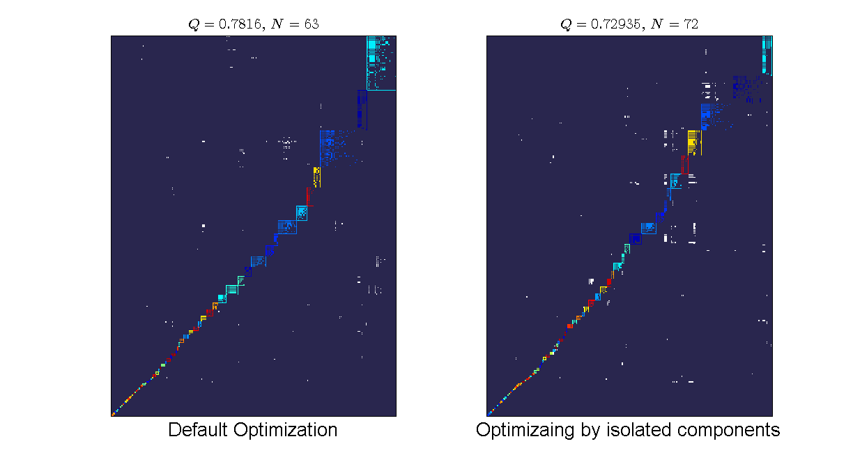
We can see that the default optimization gives a higher modularity value (we are optimizing at the entire matrix) but lower number of modules than the component optimization. By optimizing at the component level, we do not have any more the constraint of the entire network optimization and therefore it is possible to break into more modules. However, the reported value is still the value of the entire network partition.